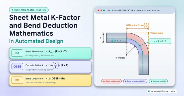
Factor of Safety in Mechanical Design: Theory vs Practice
The factor of safety is a bridge between material physics and real-world uncertainty, not an ignorance factor. This guide covers factor of safety, margin of safety and reliability, von Mises, Tresca and Modified Mohr criteria, fatigue lines, stress-strength interference, FEA singularities and two worked examples with every number computed.

Md Anamul Hasan
Mechanical Design Engineer, CSWE & PLM Project Manager
- November 8, 2026
- 25 min read
- 3 reads
- Updated November 8, 2026
The Factor of Safety is not an “ignorance factor” or an arbitrary multiplier. It is the bridge between deterministic material physics and operational uncertainty.
In introductory engineering courses, the Factor of Safety () is a single number: divide material yield strength by applied stress, and if the result exceeds the part will not break. In practice, parts sized with a textbook factor of still fail in service, while aircraft structures fly safely for decades with a factor of on limit load.
Why does this disconnect exist? Because failure in real machines is rarely a one-dimensional static overload. Components fail from multi-axial stress states, fatigue cracks that start at stress concentrations, thermal gradients, and statistical scatter in material properties. Sizing a component without knowing whether failure is governed by yielding, fracture, fatigue, buckling or variance turns the Factor of Safety into a gamble.
I work in mechanical design and CAD/PLM engineering automation, with 9+ years of experience across structural integrity, sheet metal and industrial machinery. This guide covers how to tell a design target from an achieved margin, how to pick the failure criterion for ductile and brittle materials, how to read a fatigue envelope on the Haigh diagram, and how to move from a single safety factor to a probability of failure.
The one-minute version
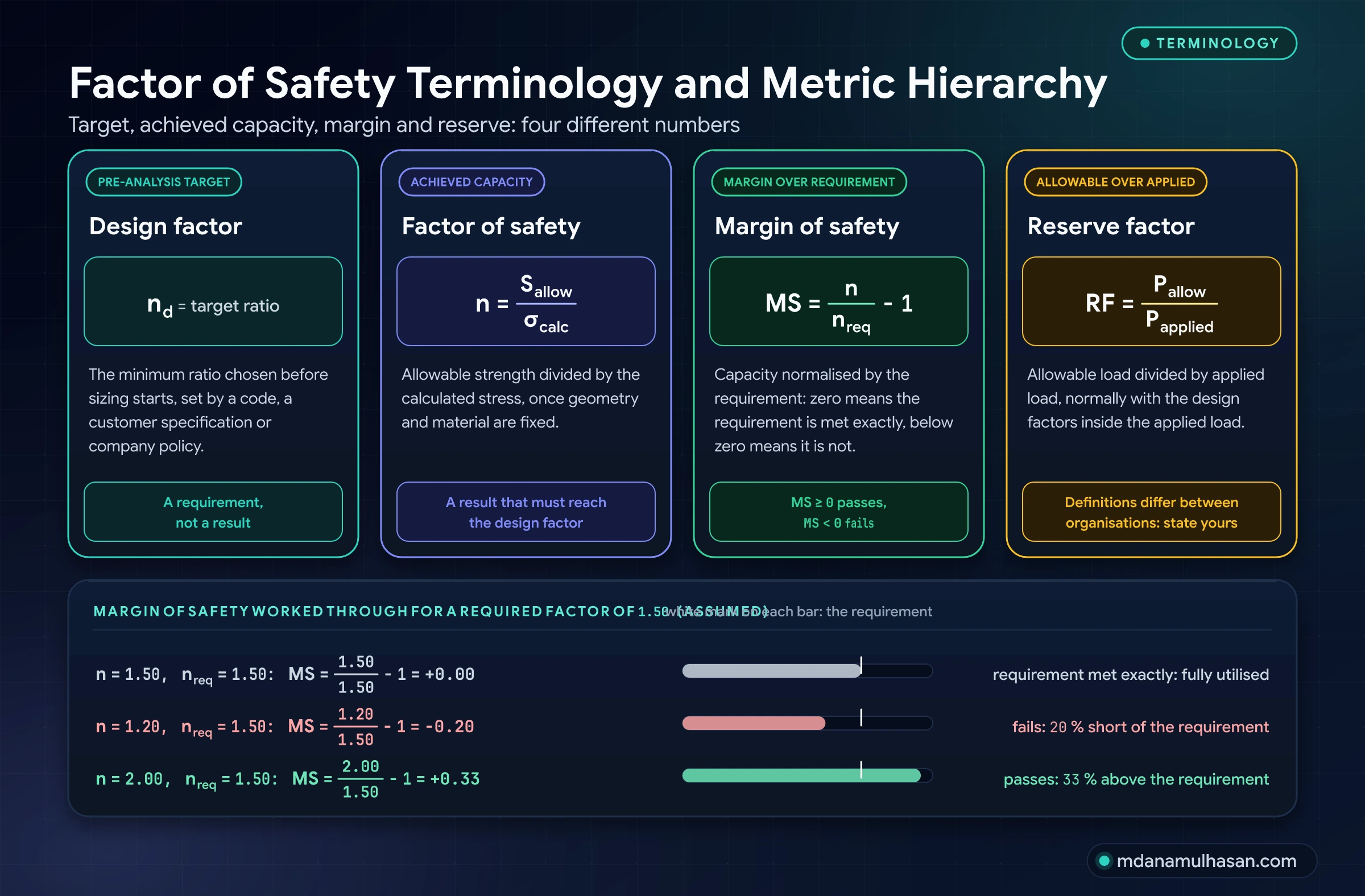
Design factor () is the minimum target ratio chosen before sizing begins, set by a code, a customer specification or company policy.
Factor of safety () is the realized ratio of allowable capacity to calculated stress after the geometry is fixed: .
Margin of safety () normalizes the achieved factor by the required one: . means the requirement is met exactly.
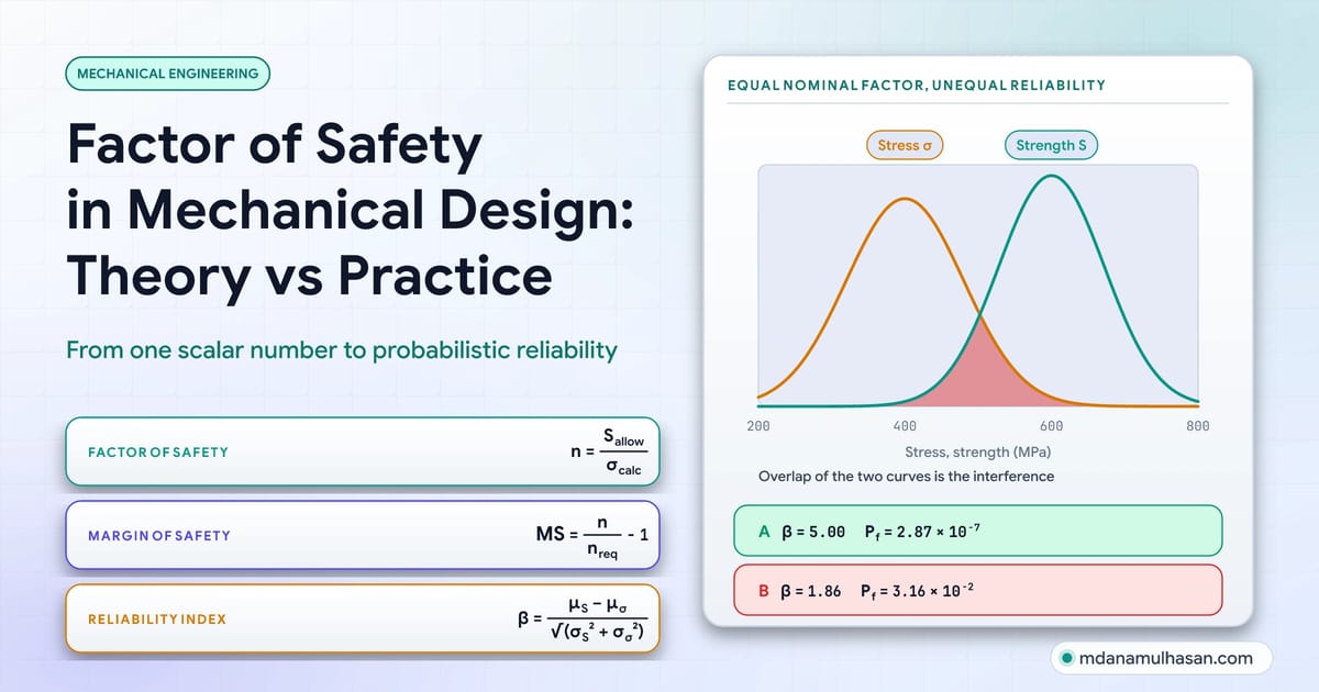
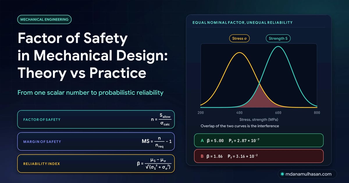
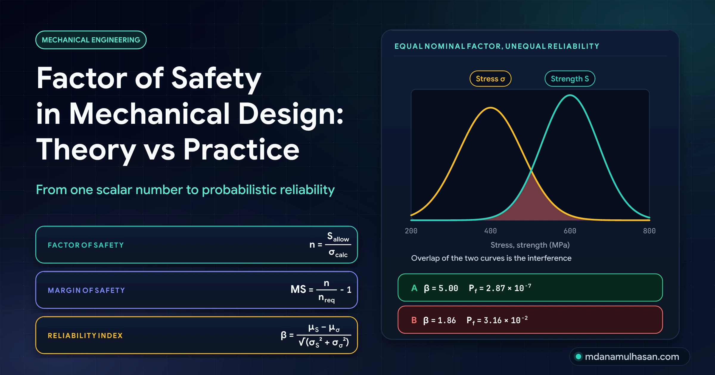
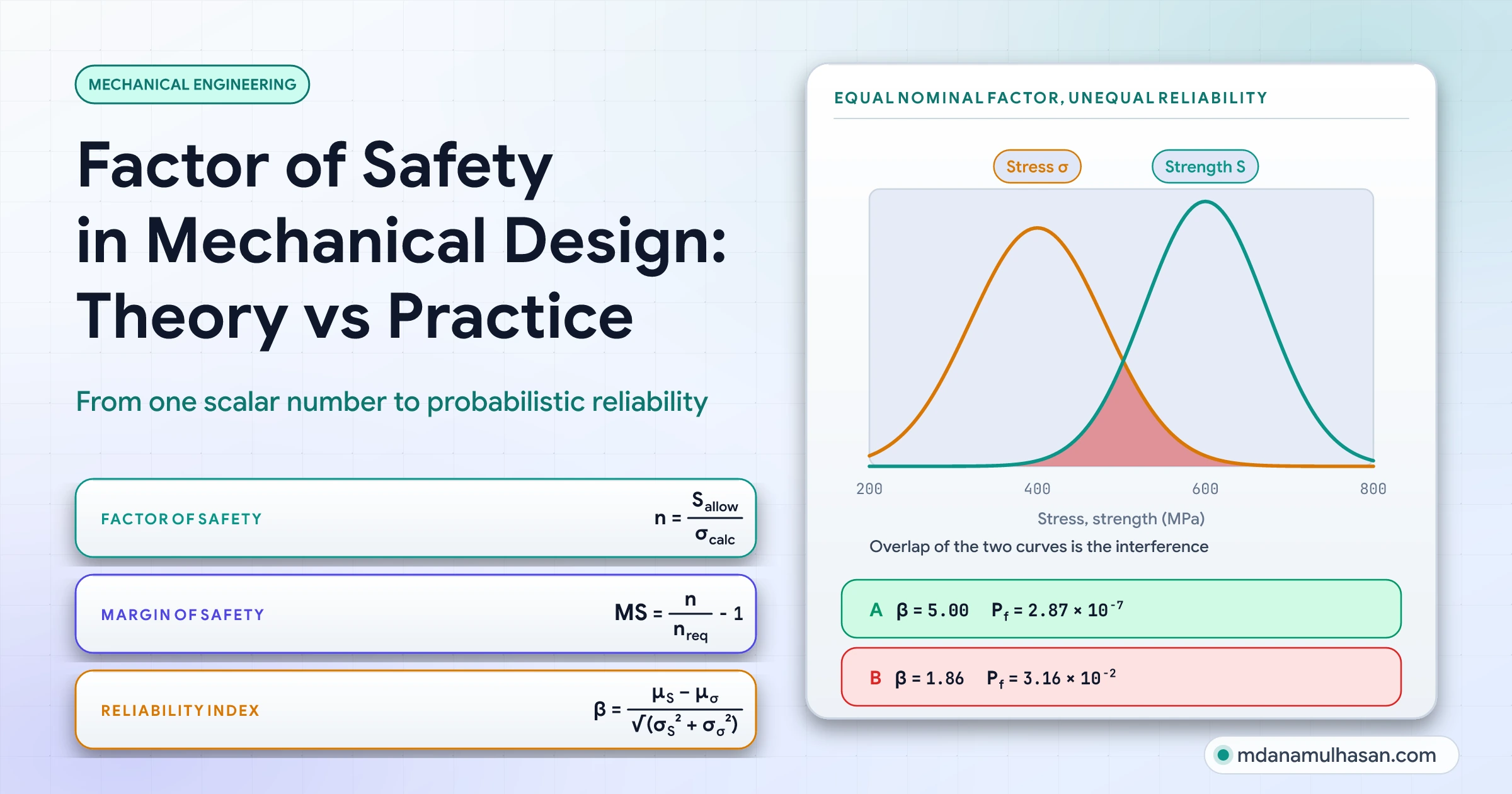
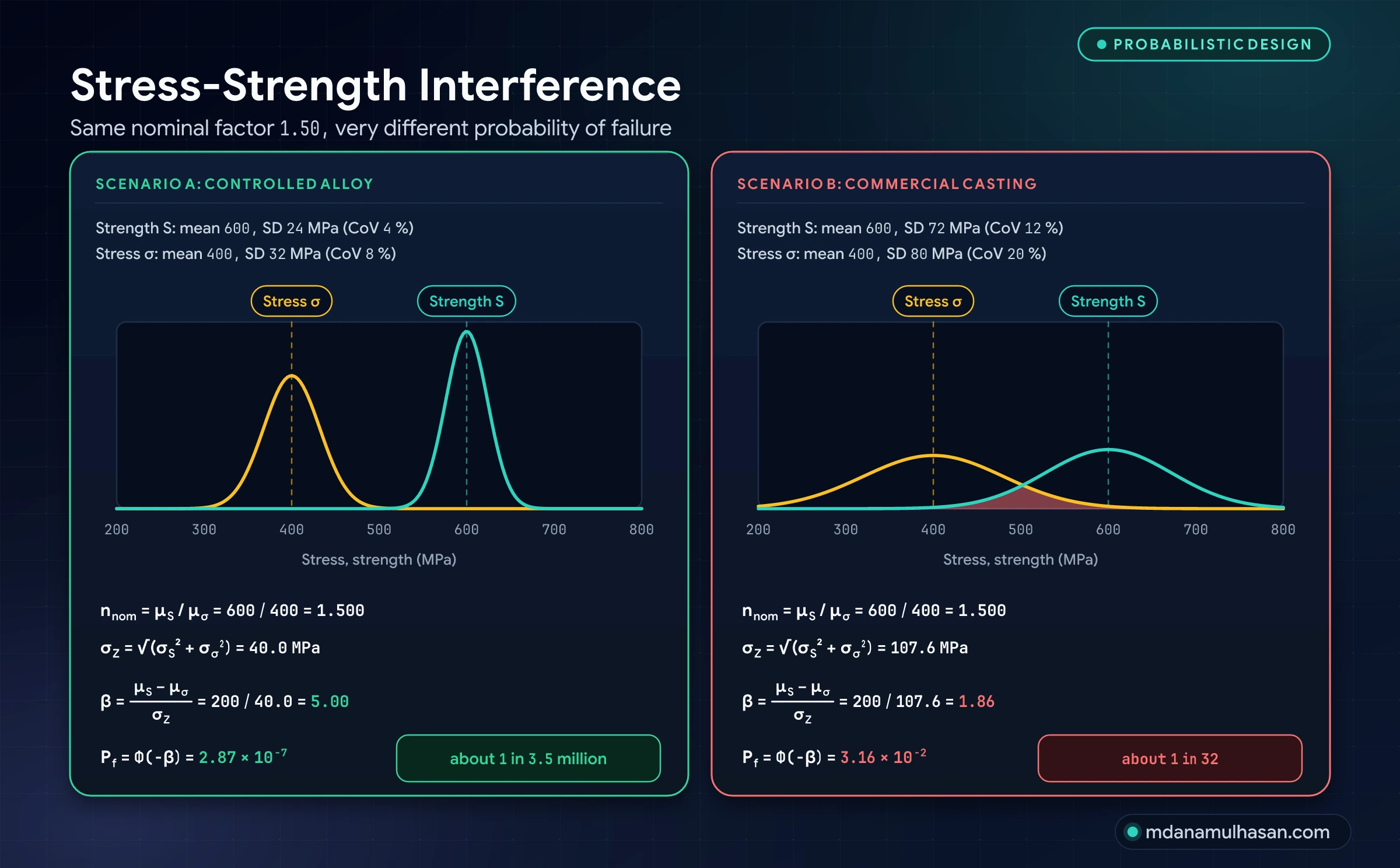
Stress-strength interference shows that the same nominal factor of can mean about failure in million () or about in (), depending on the scatter of strength and stress. The scatter values are assumptions chosen for the comparison.
The three core static and fatigue formulations:
Here is yield strength, is ultimate tensile strength, is the fully corrected endurance limit, is the von Mises stress, is alternating stress and is mean stress. All stresses and strengths are in megapascals (MPa).
Terminology and metric hierarchy
One of the most persistent sources of confusion in engineering teams is the interchangeable use of terms that have distinct definitions.
| Metric | Definition | Engineering phase | Meaning |
|---|---|---|---|
| Design factor () | Before analysis | A requirement set by a code, a specification or policy. | |
| Factor of safety () | After analysis | Capacity realized by the final dimensions and material. | |
| Margin of safety () | Verification and release | Common in aerospace reporting. Normalizes capacity against the requirement. | |
| Reserve factor () | Structural analysis | Allowable load over applied load. Definitions differ between organizations, so state yours. |
Interpreting the margin of safety ()
Reporting alone is incomplete, because it does not say what was required. The margin of safety states it:
- : the requirement is met with capacity to spare.
- : the requirement is met exactly. A margin far above zero usually means material that could be removed, but how much margin to hold is a project decision.
- : the requirement is not met. An is a shortfall against the requirement, even if the nominal factor is greater than .
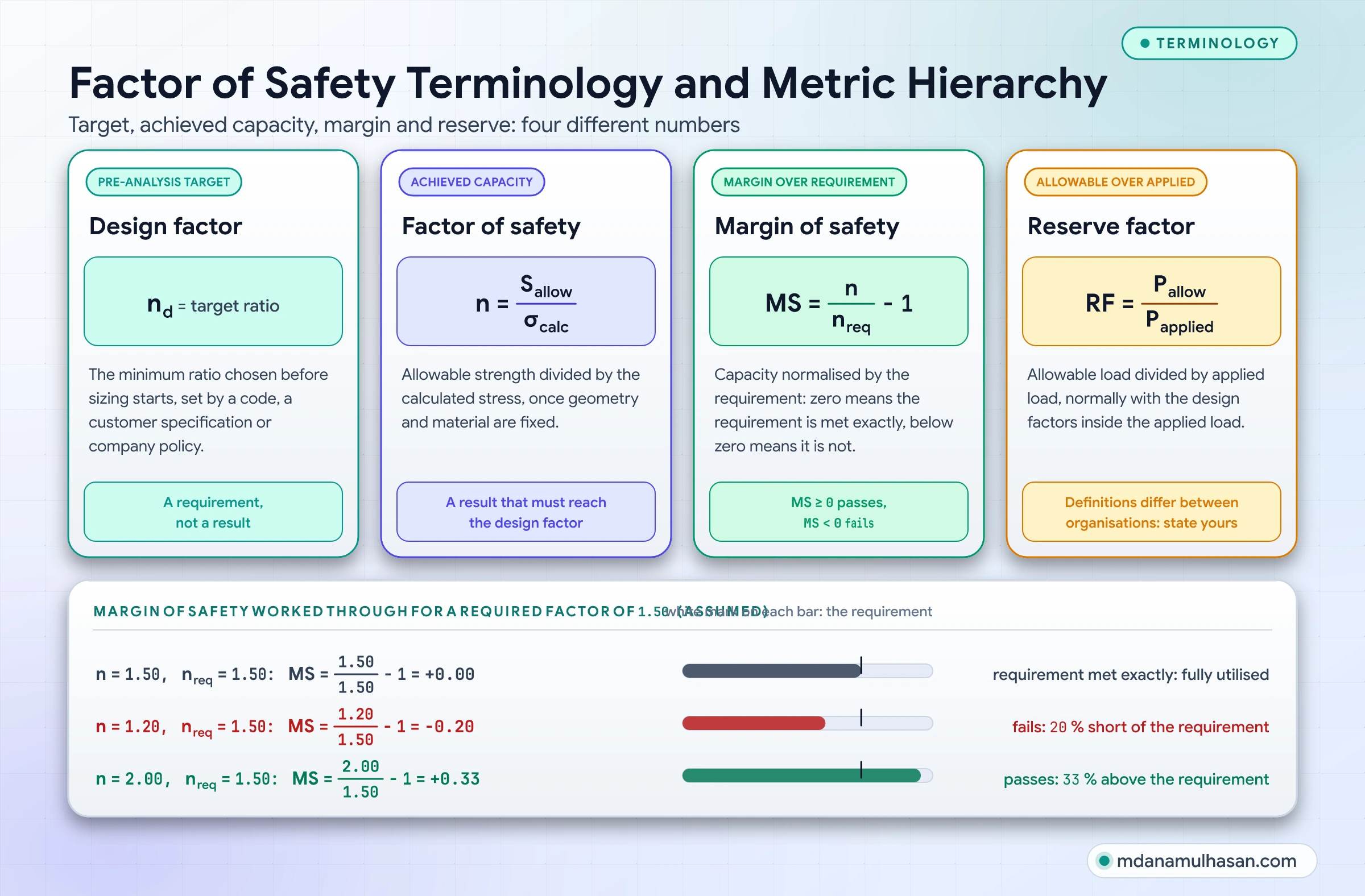
For example, if a flight bracket requires and stress analysis gives :
The bracket passes with a margin over the requirement.
Why a single scalar FoS fails in real machines
Treating the Factor of Safety as one multiplier assumes that stress scales linearly with load and that failure depends on a single stress component. Both assumptions are often false:
- Multi-axial stress states: Yielding of ductile metals is driven by distortion (deviatoric) energy, not by hydrostatic pressure. To a good approximation a steel specimen under MPa of hydrostatic compression does not yield, whereas the same steel under pure torsion yields at a shear stress of .
- Non-linear geometric effects: In columns, thin plates and slender shells the relation between load and stress is non-linear. A strut loaded to of its Euler critical load has a nominal factor of against buckling, but imperfections and load eccentricity lower the real critical load, so the true margin is smaller than the nominal ratio.
- Contact (Hertzian) stress: In rolling bearings, gears and cam-follower contacts, contact stress grows with the cube root of load for point contact and the square root for line contact. Doubling the load raises contact stress by only to , yet fatigue life falls much faster: the rating life equation of rolling bearings uses a load exponent of for ball bearings and for roller bearings (ISO 281:2007, Equations 4 and 16), so doubling the load cuts the rating life by a factor of about to .
Static yield and fracture failure envelopes
To calculate a meaningful factor under static loading, the multi-axial stress state is collapsed into an equivalent stress that can be compared with uniaxial test data. The choice of failure theory depends on whether the material yields plastically or fractures in a brittle way.
1. Ductile materials: von Mises vs Tresca
For ductile metals (structural steels, aluminum alloys, copper, titanium), yielding is driven by shear on slip planes.
Distortion energy (von Mises)
The von Mises criterion states that yielding begins when the second invariant of the deviatoric stress tensor () reaches its value at yield in simple tension:
In plane stress () this becomes:
Maximum shear stress (Tresca)
The Tresca criterion states that yielding occurs when the maximum shear stress equals the shear stress at yield in a uniaxial tensile test:
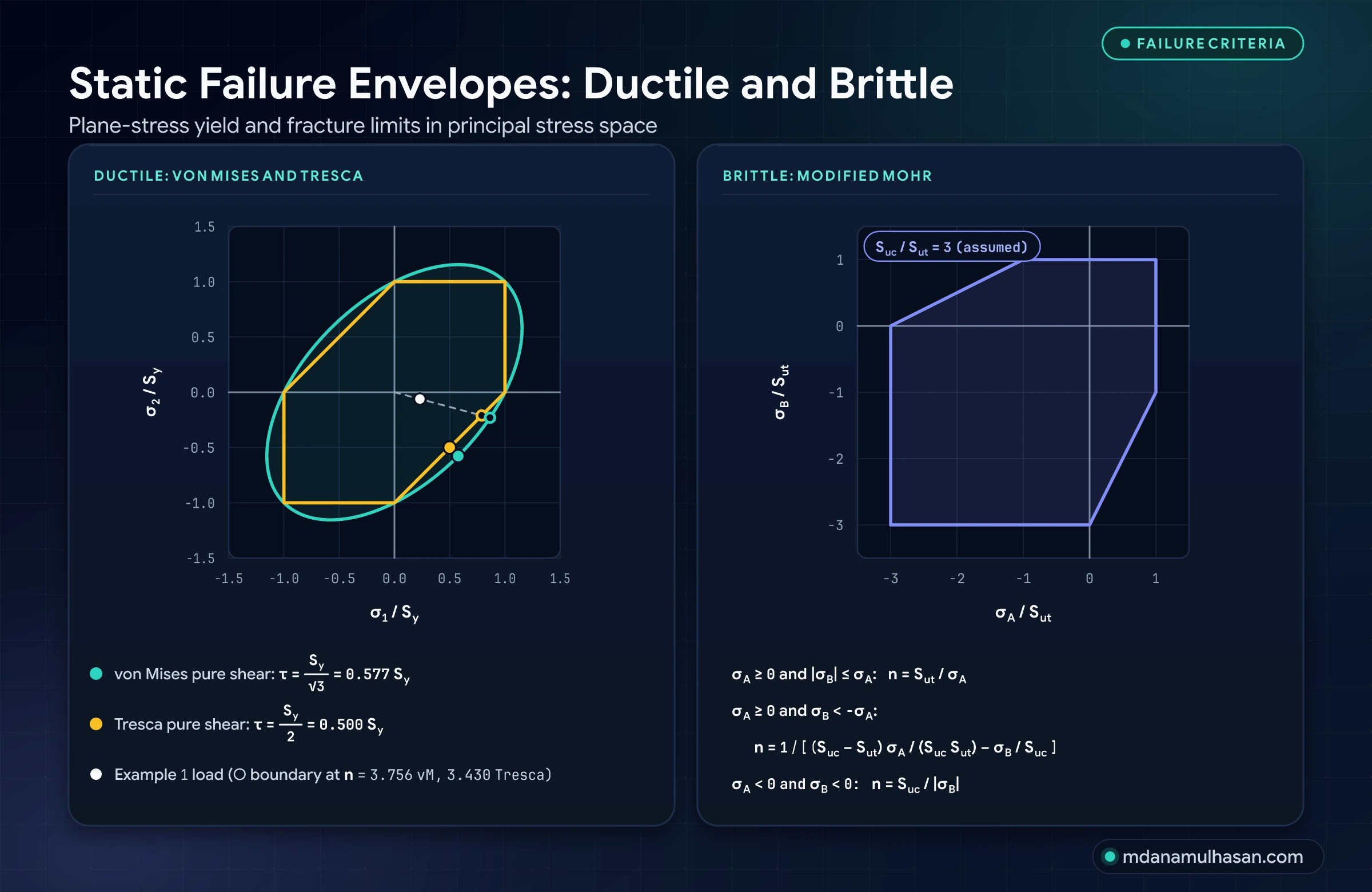
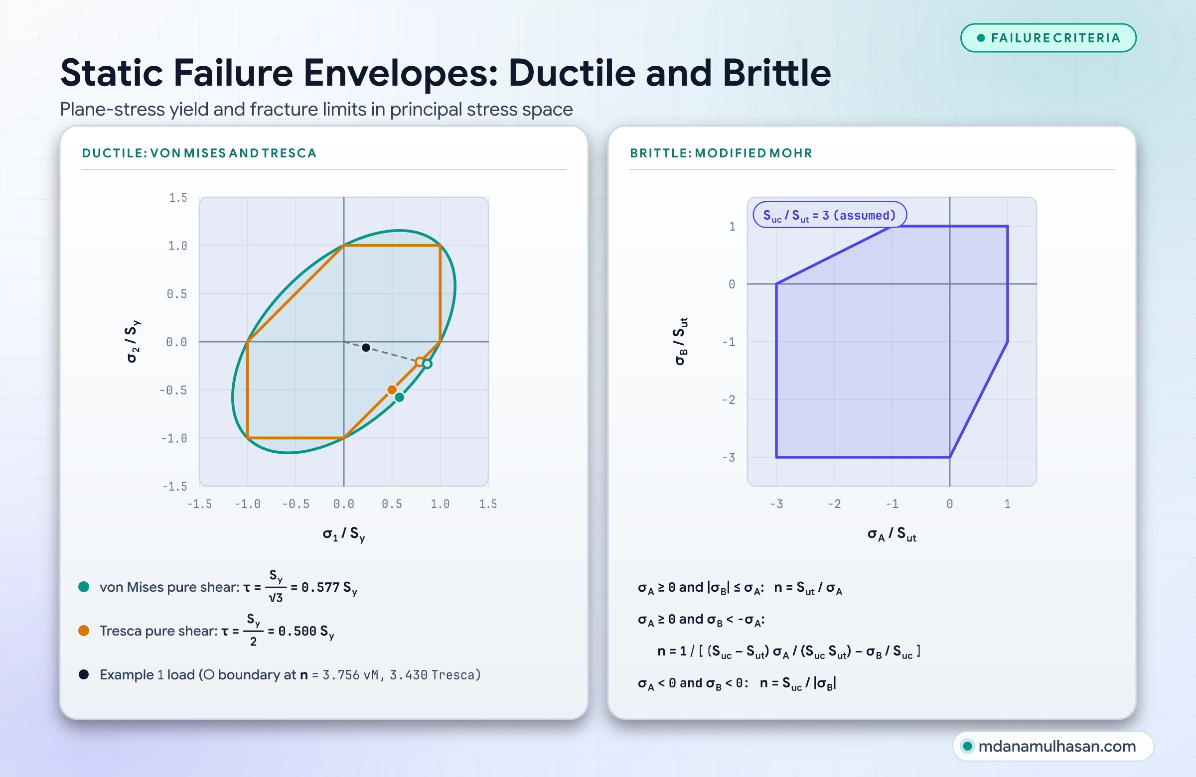
The Tresca hexagon is inscribed in the von Mises ellipse. In pure shear (), von Mises predicts yield at and Tresca at . Von Mises therefore allows a shear stress higher than Tresca, or equivalently Tresca’s allowable is lower. Codes differ in which criterion they adopt (stress intensity, which is Tresca, or von Mises): follow the one your governing code states.
2. Brittle materials: Modified Mohr
Brittle materials (grey cast iron, hardened tool steels, ceramics) show almost no plastic deformation before fracture, and their compressive strength () is several times their tensile strength ().
With the principal stresses ordered , the Modified Mohr criterion splits plane-stress space into three regions:
- When and (including both stresses tensile), tensile strength governs:
- When and , the tension-compression region applies:
- When and , compressive strength governs:
Fatigue and fluctuating loads
Fatigue is a leading cause of in-service fracture of cyclically loaded metal parts, and it occurs at stresses well below the static yield strength. Sizing shafts, connecting rods, springs or bolted joints with a static yield factor alone is one of the most dangerous oversights in mechanical design.
Resolving cyclic stress components
Any fluctuating stress history can be split into an alternating amplitude () and a steady mean ():
The Marin endurance limit modifiers
The endurance limit of a rotating-beam test specimen ( for steels with MPa) is reduced for real surfaces, sizes, loading and reliability with the Marin factors:
| Marin factor | Physical driver | How it is obtained |
|---|---|---|
| Surface condition () | Surface finish (ground, machined, hot-rolled, as-forged) | Power-law fit with coefficients for each finish |
| Size () | Diameter and the volume of highly stressed material | Fit as a function of diameter; for axial loading |
| Load () | Bending, axial or torsional loading | bending, axial, torsion |
| Temperature () | Strength at operating temperature | Ratio of tensile strength at temperature to room temperature |
| Reliability () | Target survival probability | , with the standard normal deviate (for example at ) |
These are textbook relationships (Shigley’s Mechanical Engineering Design) and were not checked against a standard.
Fatigue notch factor ()
Holes, keyways and snap-ring grooves create a theoretical stress concentration (). In fatigue the material responds with a notch sensitivity ():
Governing fatigue failure criteria
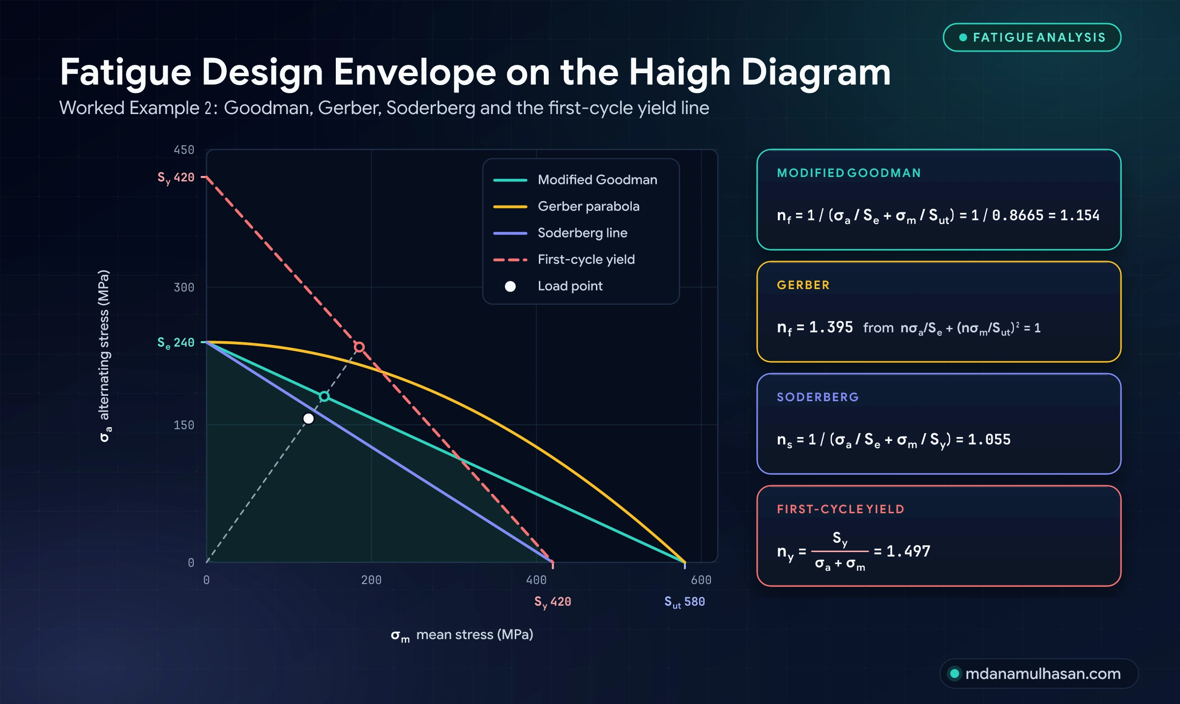
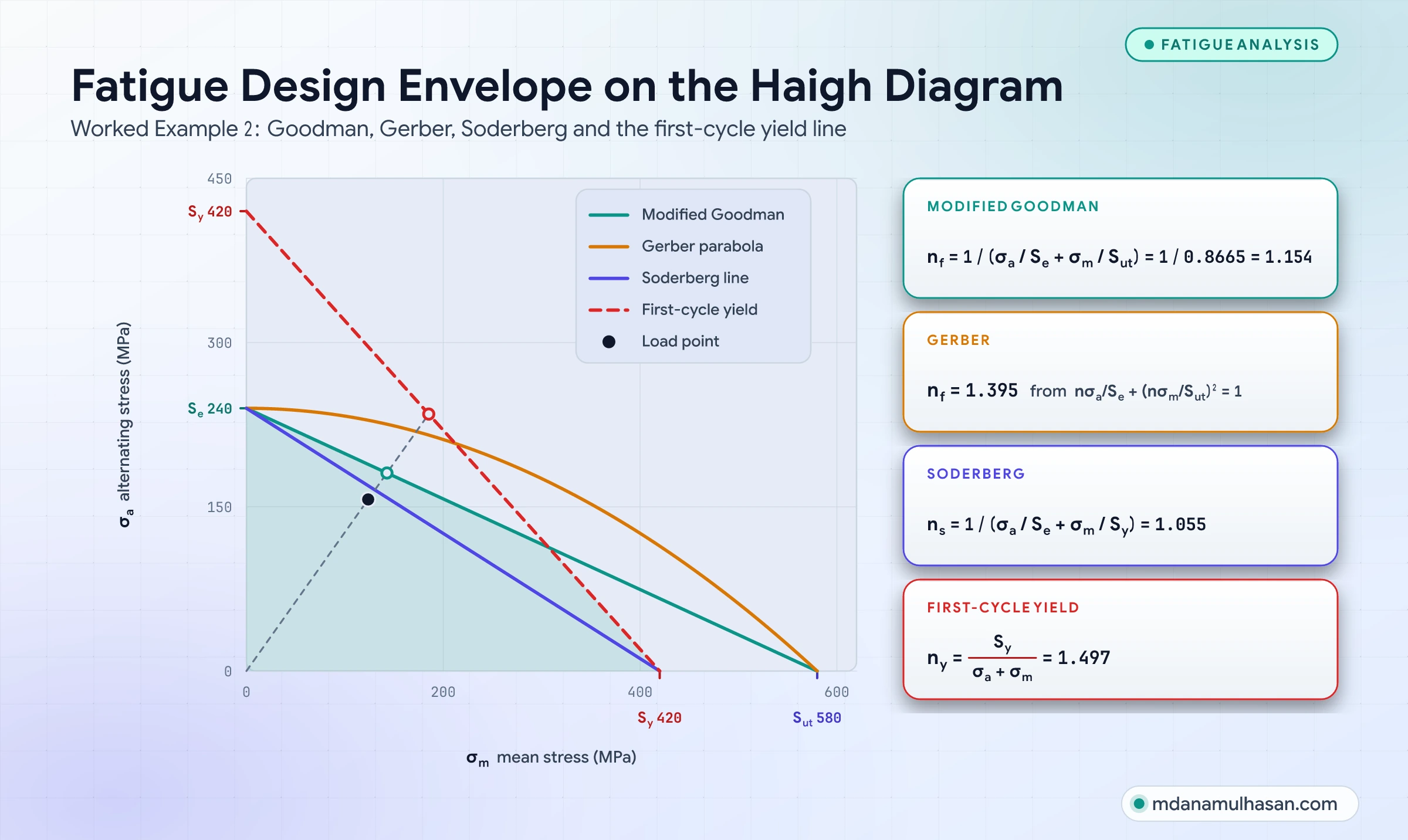
On the Haigh diagram ( horizontal, vertical) the safe boundary is defined by empirical relationships:
- Modified Goodman (common practice):
- Gerber parabola (a better fit to ductile steel data):
- Soderberg line (conservative, yield-based):
The first-cycle yield check: Even if Modified Goodman predicts , the first load cycle can yield the part if the peak stress exceeds yield. An independent static check is required:
Stress-strength interference: probabilistic reliability
A deterministic factor assumes that strength and load are fixed numbers. In reality every material lot has a distribution of strengths, and every operating environment produces a spectrum of load peaks.
Stress-strength interference replaces single numbers with probability density functions:
- Strength:
- Working stress:
The reliability index ()
Define the safety margin . For independent normal and , is also normal:
The reliability index is the number of standard deviations between the mean margin and the failure threshold ():
The probability of failure () is the area of the interference tail:
The 1.50 FoS paradox: controlled alloy vs commercial casting
Take two designs with the same nominal factor . The means and standard deviations below are assumed for the comparison:
| Parameter | Scenario A: controlled alloy | Scenario B: commercial casting |
|---|---|---|
| Mean strength () | MPa | MPa |
| Strength std dev () | MPa () | MPa () |
| Mean stress () | MPa | MPa |
| Stress std dev () | MPa () | MPa () |
| Nominal factor () | ||
| Combined std dev () | MPa | MPa |
| Reliability index () | ||
| Probability of failure () | (about in million) | (about in ) |
The comparison shows why a factor alone says little. Under Scenario A, tight material control and well-known loads give a survival probability of . Under Scenario B, scatter in casting strength and uncertain loads put more than in parts at risk, despite the same on paper.
Pugsley’s rational method
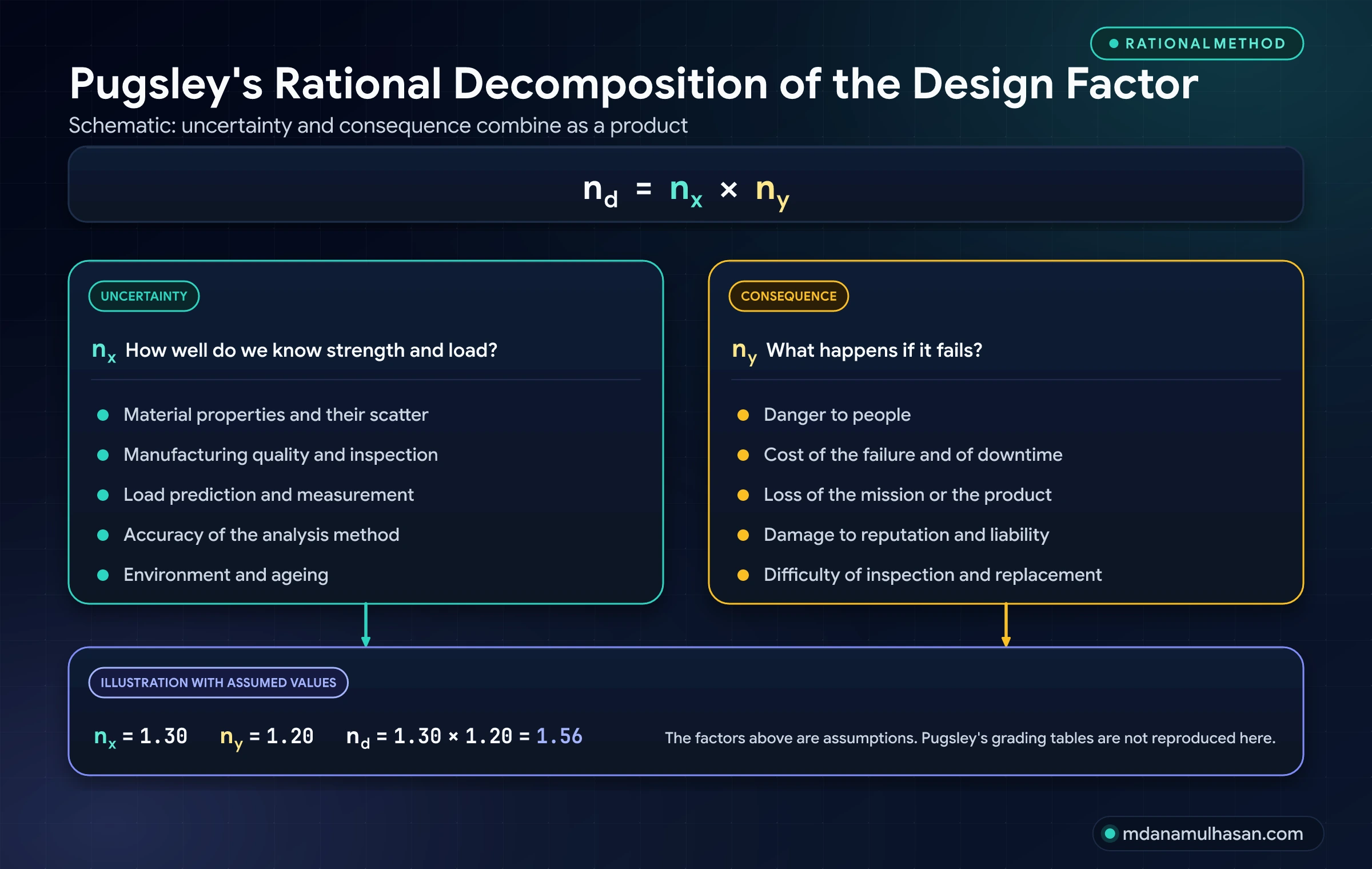
When test data is incomplete, Sir Alfred Pugsley’s rational method gives a structured way to choose the design factor: split it into a part for uncertainty and a part for consequence, then multiply them:
Factor : uncertainty
grows with how little is known about strength and load. It collects the scatter of material properties, the quality of manufacture and inspection, the accuracy of load prediction and measurement, the accuracy of the analysis method, and the environment and ageing.
Factor : consequence
grows with what a failure costs. It collects danger to people, the cost of the failure and of downtime, loss of the mission or product, damage to reputation and liability, and the difficulty of inspecting or replacing the part.
Pugsley published graded tables for these characteristics. They are not reproduced here because the source is not in the standards library used for this article. As an illustration only, assuming and gives . The method makes the reasoning explicit and reviewable, which a bare “use ” does not.
Industry codes and standards comparison
Design codes reflect decades of failure experience, balancing safety against cost and weight.
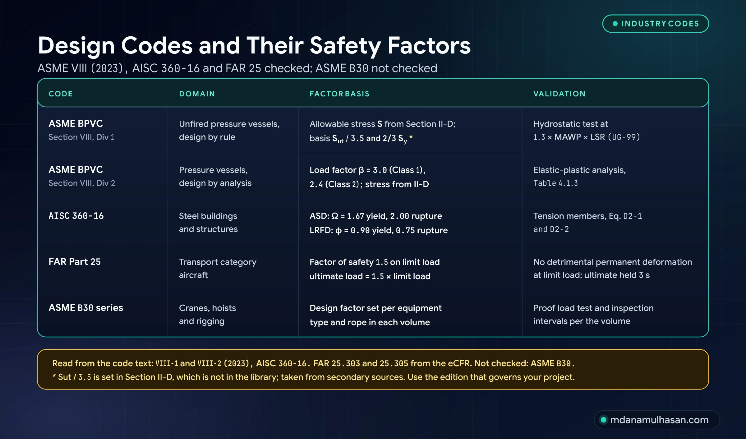
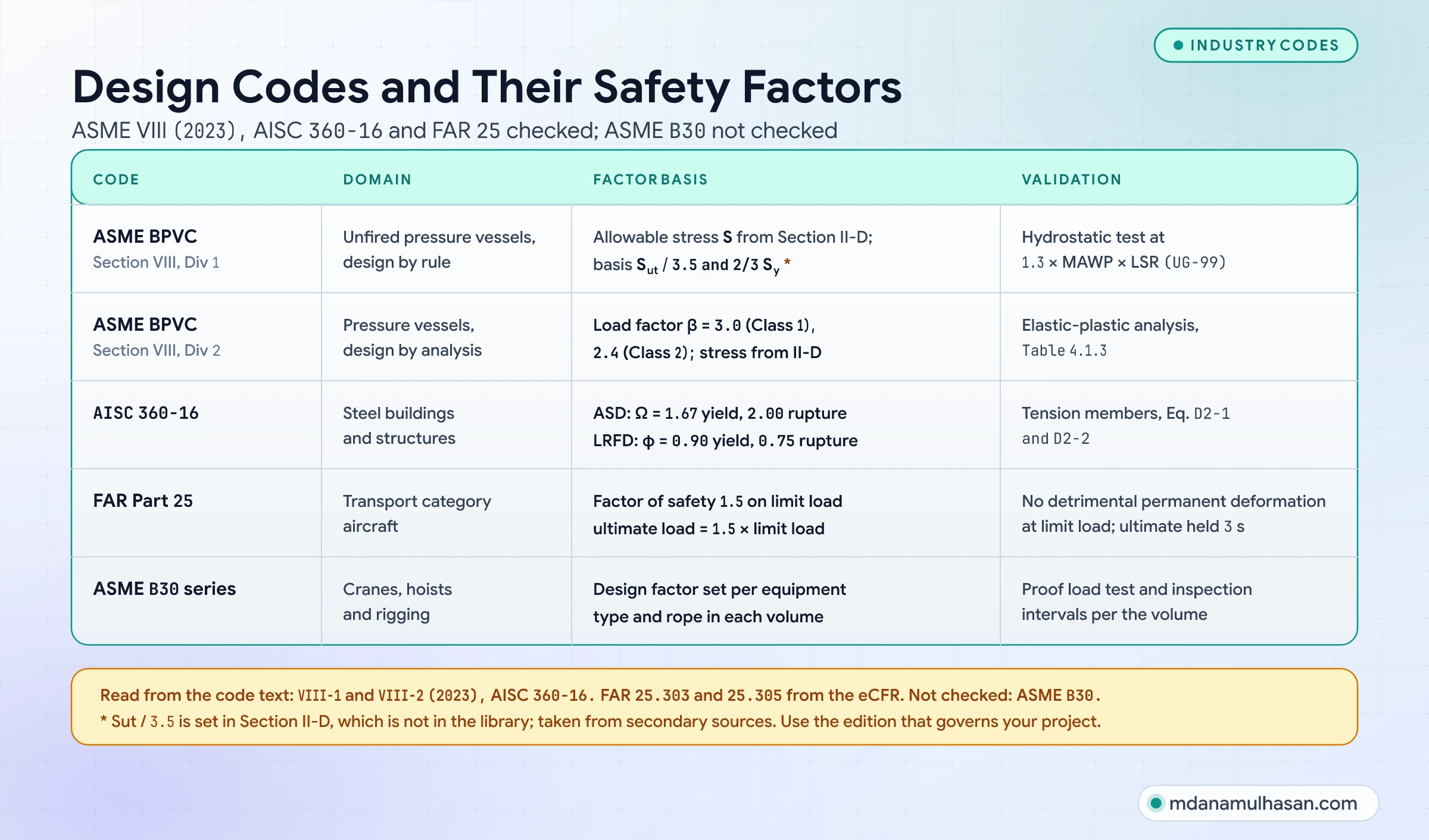
This article is not endorsed by or affiliated with ASME, AISC, ISO or the FAA. Values are paraphrased or computed for explanation, no tables or figures of the standards are reproduced, and the published standard governs.
Checked against the code text: ASME BPVC VIII-1 and VIII-2 (2023 edition) and AISC 360-16 (read from the PDFs), and FAR 25.303 and 25.305 (eCFR). Not checked: ASME B30, and the and allowable-stress bases, which are set in ASME Section II, Part D and were taken from secondary sources. Use the edition and clauses that govern your project.
| Code | Application | Factor basis | Validation |
|---|---|---|---|
| ASME BPVC Section VIII Div 1 | Unfired pressure vessels, design by rule | Allowable stress comes from Section II, Part D. Its basis is the lesser of and (secondary sources) | Hydrostatic test at , where LSR is the lowest stress ratio of the pressure-boundary materials (UG-99) |
| ASME BPVC Section VIII Div 2 | Pressure vessels, design by analysis | Elastic-plastic load factor (Class 1) or (Class 2); allowable stress from Section II, Part D (Table 2A for Class 1, Table 5A for Class 2) | Table 4.1.3 sets the load and test factors |
| AISC 360-16 | Steel buildings and structures | Tension members (D2): ASD (yielding), (rupture). LRFD (yielding), (rupture) | Required strength comes from the governing load standard; AISC 360 uses for load-test rating |
| FAR Part 25 | Transport category aircraft | Factor of safety applied to the prescribed limit load (25.303) | No detrimental permanent deformation at limit load; ultimate load held for at least seconds (25.305) |
| ASME B30 series | Cranes, hoists and rigging | Design factor set per equipment type and rope in each volume (not checked) | Proof load test and inspection intervals per the volume (not checked) |
The FEA stress singularity trap
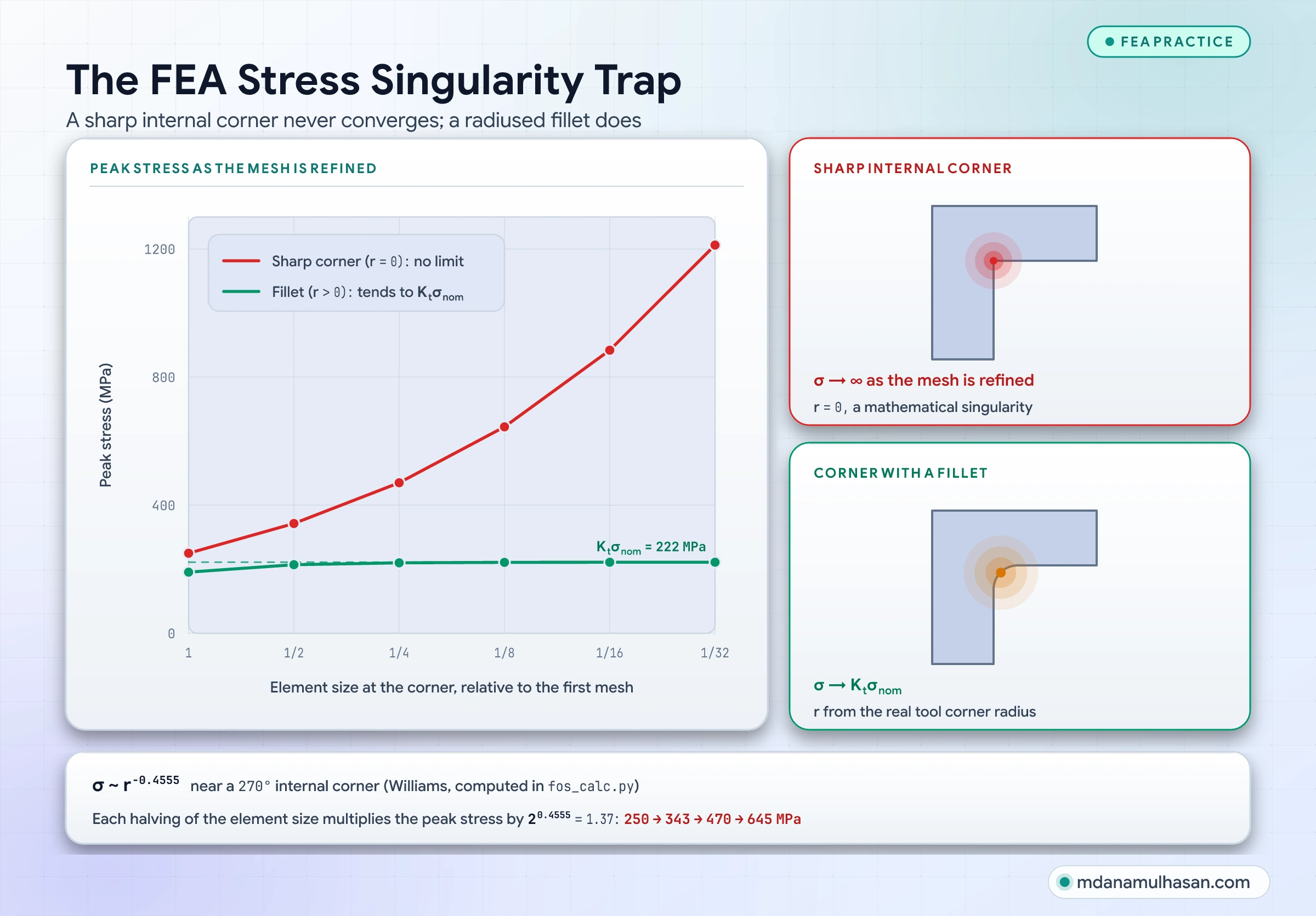
Finite element programs solve linear elasticity, where a perfectly sharp internal corner has a radius of zero (). In that model the stress at the corner is theoretically infinite (), so the number the program reports there depends on the mesh, not on the part.

Recognizing a singularity vs a true stress concentration
When you refine the mesh:
- At a true notch modeled with its real radius (), the peak stress converges to a fixed value ().
- At a singularity (a sharp internal corner, a point load or a rigid constraint) the peak stress keeps climbing. For a internal corner the stress varies as , so every halving of the element size multiplies the peak by : for example MPa over three refinements. The exponent is computed from Williams’ eigenvalue equation in the calculation module described below.
Engineering rules for FEA safety factors
- Model the radius that the tool or process actually produces: Do not leave internal corners in high-stress zones at zero radius.
- Stress linearization: On a section that carries primary load, define a stress classification line across the thickness and split the stress into membrane (), bending () and peak () parts. Compare membrane and membrane-plus-bending stress with the code allowables. For example, in ASME Section VIII Division 2 the elastic limits are and , with the allowable stress (not checked against the code text):
- Neuber’s rule for local plasticity: In a ductile material, a peak above yield does not mean failure; the surface layer yields locally and sheds load to the surrounding elastic material. Neuber’s rule (, with and the elastic nominal values) estimates the local stress and strain.
Worked Example 1: Transmission shaft under combined bending and torsion
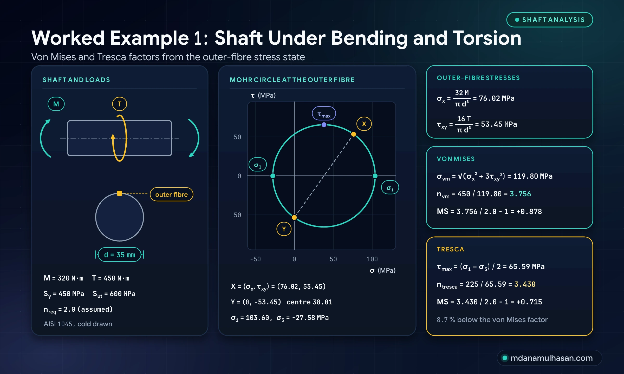
A solid shaft of cold-drawn AISI 1045 steel with diameter mm carries a steady bending moment and torque:
- Bending moment:
- Torque:
- Yield strength: MPa, ultimate strength: MPa
- Required factor: (assumed)
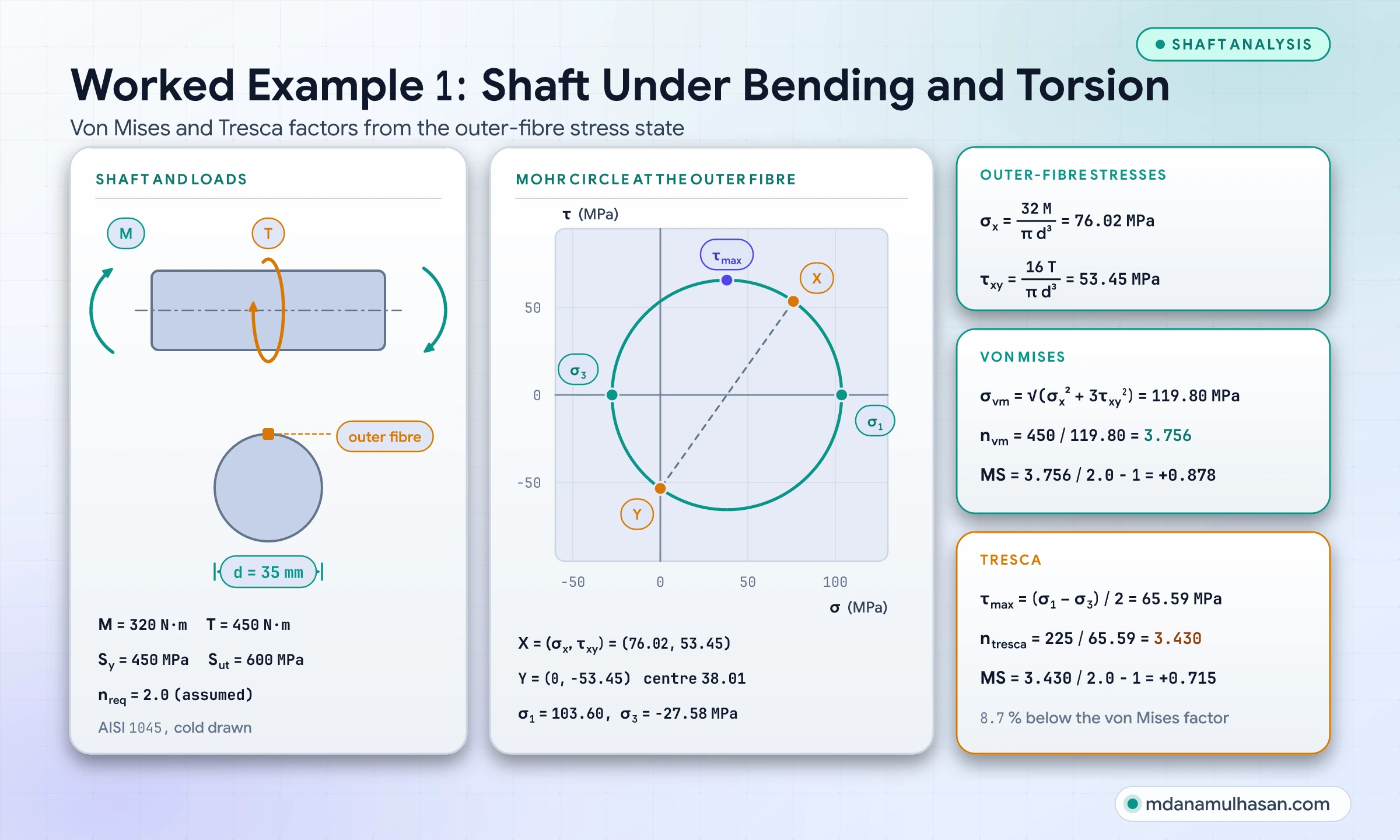
Step 1: Outer-fibre stresses
Bending stress at the outer surface:
Torsional shear stress at the outer surface:
Step 2: Von Mises factor of safety
Step 3: Tresca (maximum shear) factor of safety
Principal stresses at the outer fibre:
Tresca gives a factor lower than von Mises ( vs ). Both clear the assumed requirement comfortably.
Worked Example 2: Notched arm under fatigue
A steel machine arm with a fillet notch carries fluctuating bending. The inputs are assumed for the example:
- Nominal alternating stress: MPa
- Nominal mean stress: MPa
- Notch: , notch sensitivity
- Fully corrected endurance limit: MPa
- Yield strength: MPa, ultimate strength: MPa
- Required factor: (assumed)
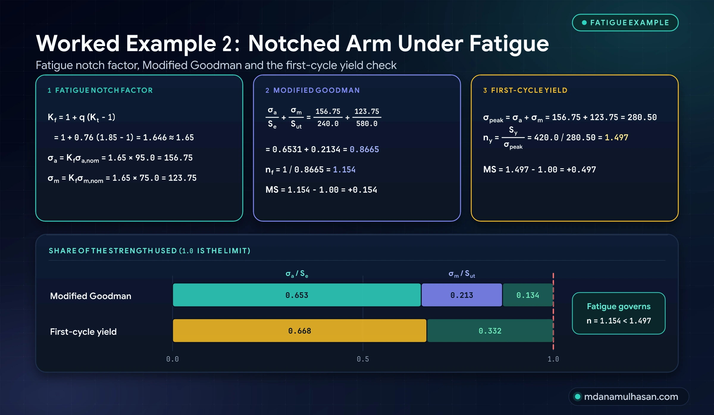
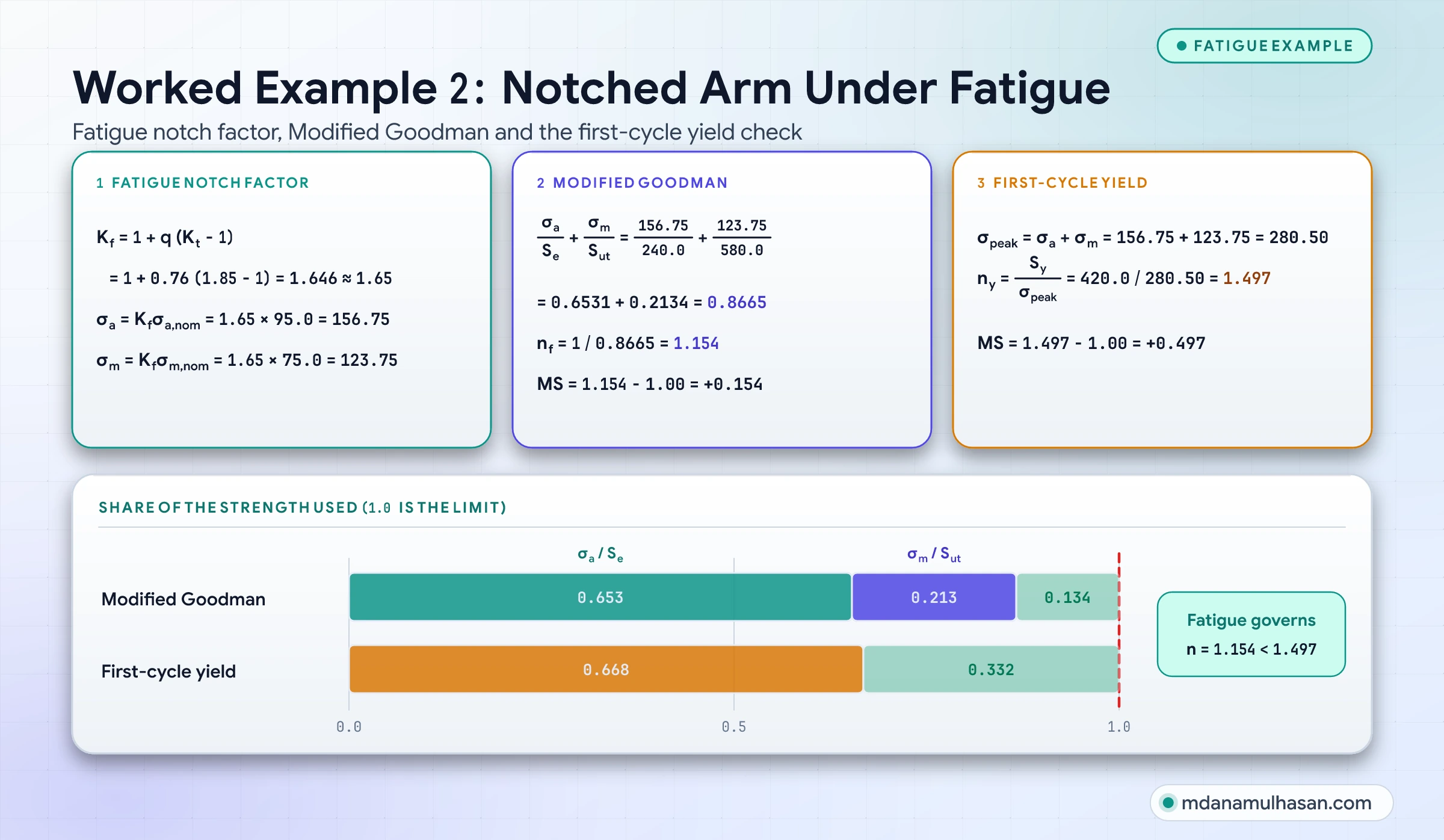
Step 1: Effective notch stresses
Step 2: Modified Goodman factor
For comparison, Gerber gives and Soderberg for the same stresses.
Step 3: First-cycle yield check
The governing factor is : fatigue, not static yield, limits this arm. With against the assumed requirement, the arm is predicted to survive indefinitely at this load, provided the steel has a fatigue endurance limit and is realistic for the surface and size.
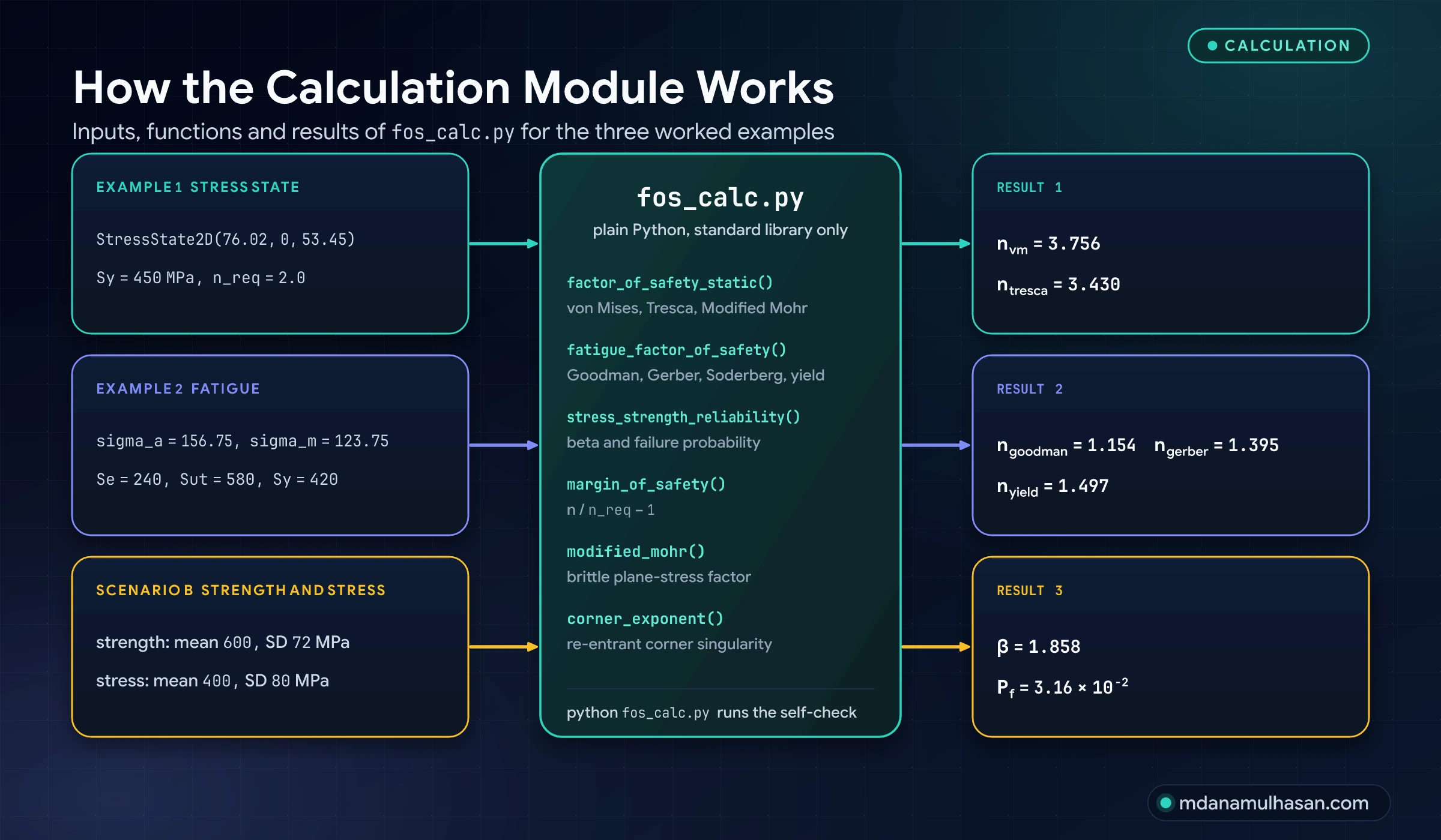
How the numbers in this article were calculated
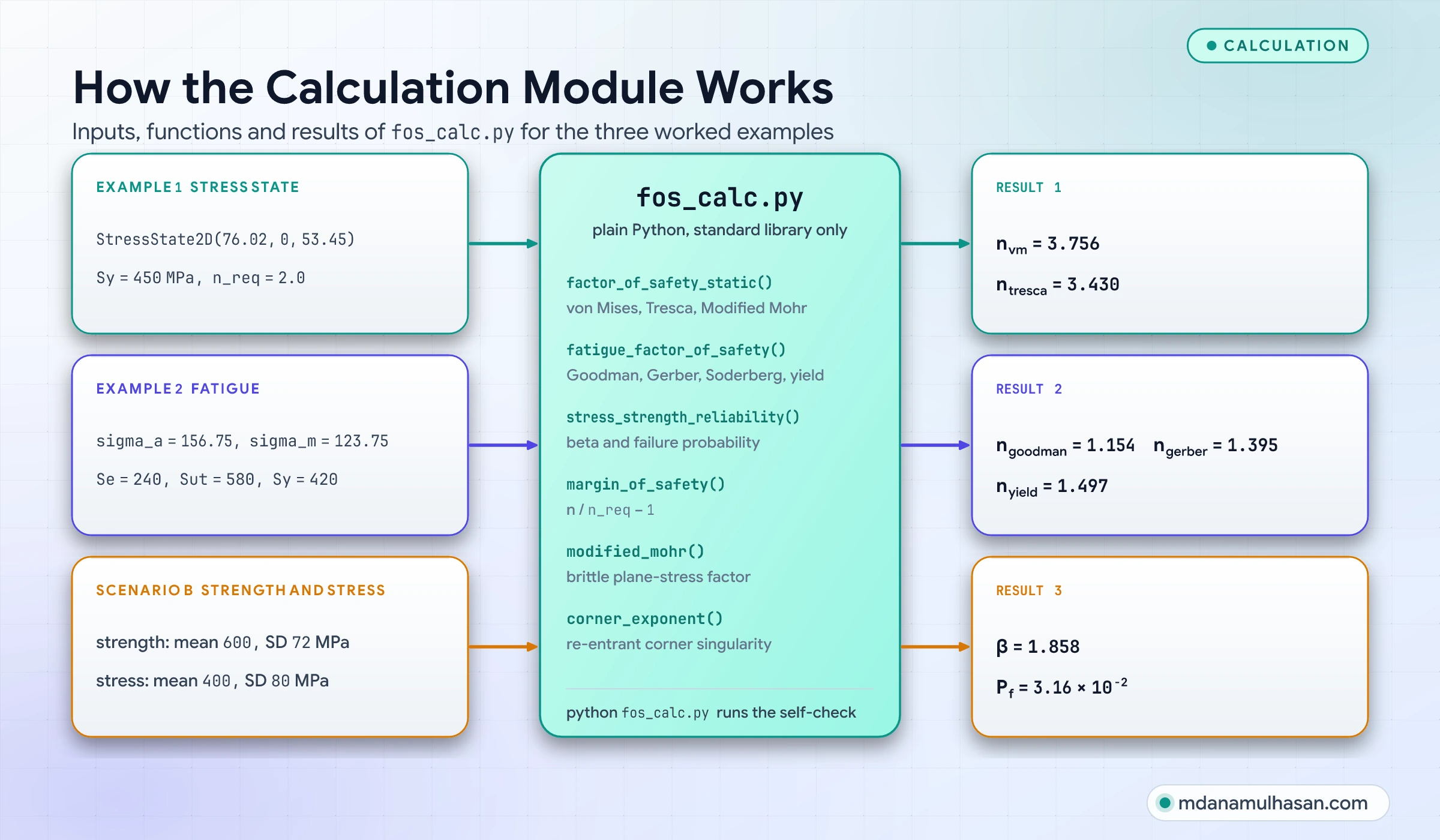
Every worked number, curve and plotted point comes from one short Python module kept with the source files of this article. It holds the failure criteria, the fatigue limit lines, the margin of safety, the stress-strength interference and the corner singularity exponent, and it checks the worked examples against the numbers printed here. The figures are generated from the same module, so the text and the pictures cannot drift apart.
The safety factor pipeline
To keep safety factor errors from reaching production drawings, careful design teams work through five stages in order.
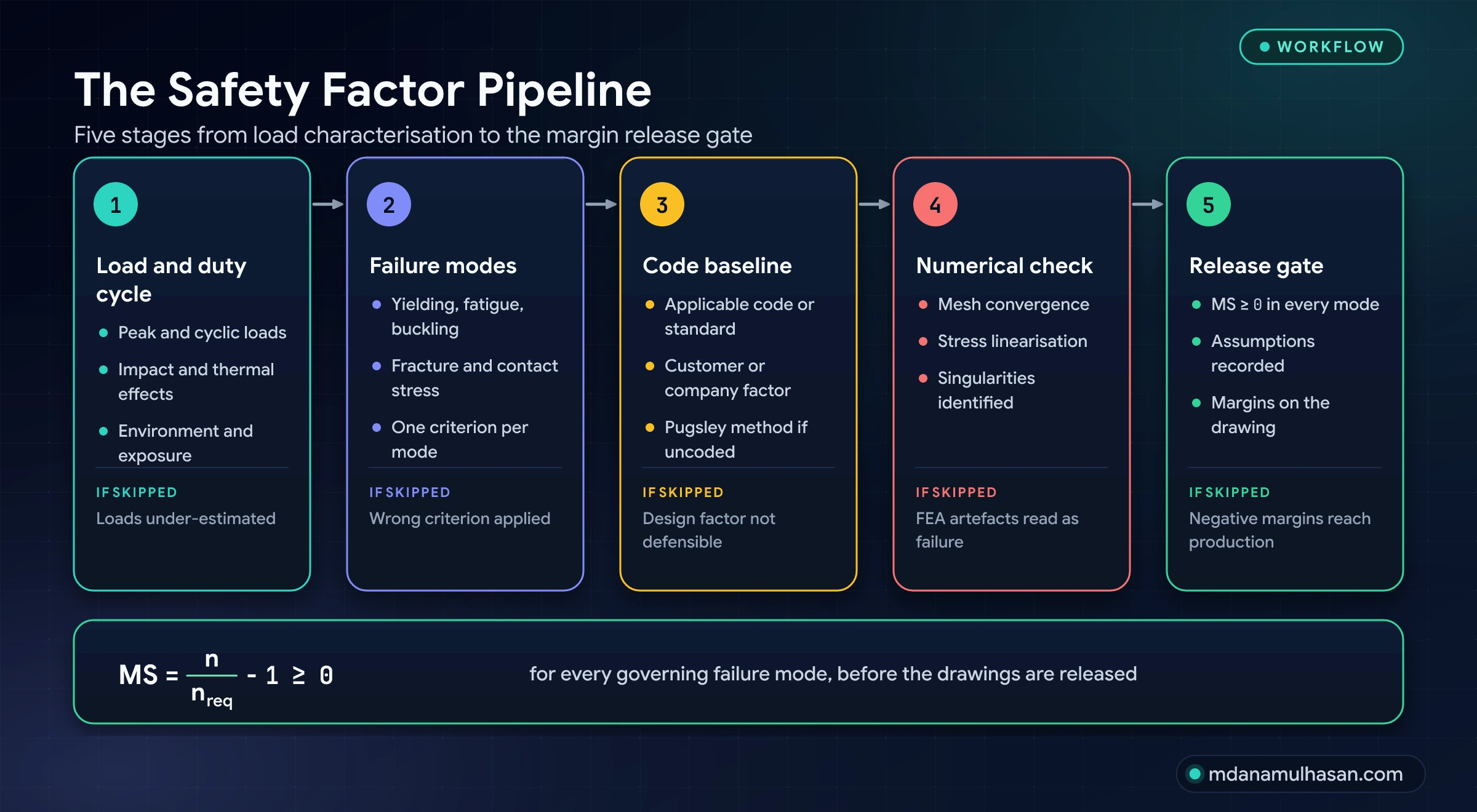
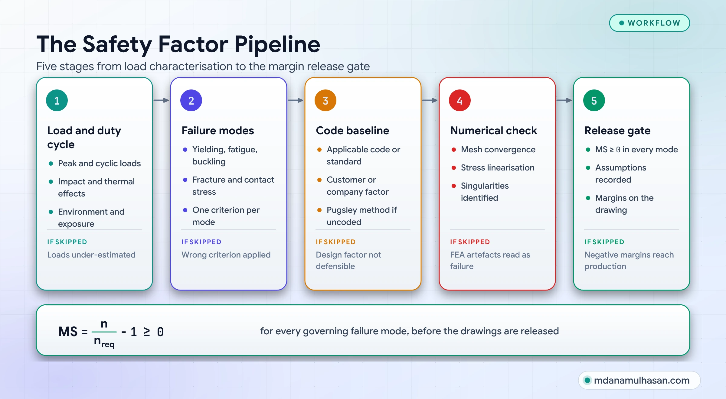
- Operating load and duty cycle: Measure or model peak loads, cyclic frequency, impact factors, thermal expansion and environmental exposure.
- Failure mode mapping: List every physical failure mechanism: yielding, fatigue, brittle fracture, buckling, contact fretting or creep. Never apply a static yield criterion to a fatigue-dominated load path.
- Code and design factor baseline: Determine whether an ASME, AISC, FAA or ISO requirement governs. For machinery with no governing code, use a structured method such as Pugsley’s to set a defensible .
- Numerical verification: Run finite element analysis with mesh convergence checks. Identify singularities, linearize stresses across critical sections and confirm the nominal stresses.
- Margin release gate (): Confirm that the margin of safety is non-negative for every governing failure mode before signing off manufacturing drawings.
Common mistakes to avoid
- Using the safety factor as an “ignorance factor”: Multiplying an uncertain load by does not protect against fatigue if the cyclic mean stress already exceeds the endurance limit. Quantify uncertainties separately.
- Confusing the design factor with the achieved factor: “The design factor is ” describes the requirement, not what the manufactured part achieves. Report the achieved margin of safety.
- Reading an FEA singularity as material failure: Rejecting a sound casting because an unradiused interior corner shows a red peak stress wastes engineering time. Model the real radius or linearize the stresses.
- Ignoring the cyclic mean stress: Checking only the alternating stress against the endurance limit misses the effect of a tensile mean stress.
- Treating all factors as equally reliable: With the assumed scatter of this article, a factor of gives about failure in million for a controlled alloy and about in for a casting with large scatter.
Quick engineering checklist
Before signing off a detail drawing or a structural analysis report, verify the following:
- Has every governing failure mode (yielding, fatigue, buckling, contact pressure) been checked independently?
- Is the failure criterion matched to material ductility (von Mises or Tresca for ductile, Modified Mohr for brittle)?
- Have internal corners in high-stress zones been modeled with the radius the process actually produces?
- Have FEA stresses been checked for mesh convergence (diverging singular peaks vs converged values)?
- For fluctuating loads, have the Marin surface, size and reliability factors been applied to the endurance limit?
- Has the first-cycle yield check () been done on every fatigue check?
- Has the margin of safety () been computed and confirmed ?
- Does the design satisfy the applicable codes and standards, read from the governing edition?
- Have material scatter and load uncertainty been reviewed with Pugsley’s method or stress-strength interference?
- Are inspection, non-destructive testing and maintenance intervals stated on the drawings?
Frequently Asked Questions
What is the exact difference between Factor of Safety and Margin of Safety?
The Factor of Safety () is the ratio of allowable capacity to working stress (). The Margin of Safety () is the fraction of capacity above the required factor (). If a code requires and the part achieves , the factor is and the margin of safety is ( above the requirement).
When should I use Tresca instead of von Mises?
Use von Mises for ductile metals (steels, aluminum, copper) when you want the best match to multi-axial test data. Use Tresca when the governing code requires it, or as a conservative hand check: it predicts yield at a lower shear stress ( against in pure shear).
Why do aircraft structures use low safety factors?
Weight is critical, so a factor of or would leave little payload. For transport aircraft the factor is on limit load. The reliability comes from other controls: extensive non-destructive testing, certified material traceability, measured flight loads, test programs and scheduled inspection.
How do I handle sharp re-entrant corners in FEA that show a very low safety factor?
A sharp internal corner () is a mathematical singularity: the stress tends to infinity whatever the material strength. Model the real manufacturing radius, read nominal stresses a few element sizes away from the corner, or linearize stresses across the section.
What is the difference between limit load and ultimate load?
Limit load is the maximum load expected in service; the structure must carry it without detrimental permanent deformation ( on yield). Ultimate load is the limit load multiplied by the factor of safety ( for transport aircraft); the structure must carry it for at least seconds without failure, even if some local yielding occurs.
Does a Factor of Safety of 2.0 mean a part can carry twice the load?
Only when stress is directly proportional to load. In buckling-sensitive columns, thin shells and contact pairs (gears, bearings), doubling the load raises stresses or the failure probability non-linearly.
How do I calculate the Margin of Safety under combined loading?
For combined axial tension, bending and torsion, form stress ratios . For a linear interaction, . For a quadratic interaction of two ratios, . The correct interaction equation depends on the failure mode and the governing method, so confirm it for your case.
What is the relationship between the Factor of Safety and the reliability index ?
The nominal factor is the ratio of mean strength to mean stress (). The reliability index also contains the standard deviations: . With no scatter, any would mean certain survival; with large scatter, a design with can still fail often when is low ( gives about failures).
Verdict and call to action
A high Factor of Safety is not a substitute for engineering. It cannot compensate for the wrong failure theory, a neglected mean stress, an FEA singularity read as a real peak, or unexamined scatter in material and load.
Treat the Factor of Safety as what it is: a calibrated tool that links deterministic models to operating reality. Set the design factor () from a code or a structured method, check multi-axial stresses against the right yield and fatigue envelopes, separate numerical singularities from real concentrations, and release the design only when for every governing failure mode.
Md Anamul Hasan is a mechanical engineer and CAD/PLM systems specialist with 9+ years of experience in structural integrity, mechanical design automation and digital engineering governance.

Written by Md Anamul Hasan
Mechanical Design Engineer, CSWE & PLM Project Manager
Specializing in mechanical design automation, CAD API scripting (SolidWorks, NX Open), and Teamcenter PLM workflow engineering.